Modelling pendulums and chaotic systems
Steven Fowler (see more projects here)
This simulation focuses of modelling pendulum systems with the future intention of implementing a control feedback system. Consequently, a function was written where time-dependent ODE systems can be solved in a step-wise manner.
What I did
- Wrote a time-dependent ODE function that can be solved in a step-wise manner.
- This was based on Sergey Royz ODE solution
- Modifications were made of my implementation and future use in feedback systems
- Accuracy of 4th order Runge-Kutta method was briefly explored for an ideal system
- The general model for 4 pendulum systems were derived
- These models were used to generate the derivative functions for the ODE function
- Simulation of the 4 pendulum systems were processed and animated
Why I did it
I've been fascinated with control systems since seeing an inverted pendulum on a cart during a university open day. Although I studied control feedback systems I've never modelled this classic example, so this is the start of my inverted pendulum on a cart simulation.
What I learnt
- The method used to implement the time-dependent ODE function works by selecting the numerical method and supplying a differential function. This is a nice approach that gives flexibility for use in other projects.
Show code
# Imports and generic settings
import numpy as np
import matplotlib.pyplot as plt
from matplotlib import animation
from matplotlib import patches
from IPython.display import HTML
Time dependent ODE solver
The following code is a time-dependent ODE function where the system can be solved by defining its differentials in a function, selecting the numerical method and then iterating in a step-wise manner.
Show code
# Reference: https://www.kaggle.com/code/zjor86/ode-solver

def ODE_to_solve(initial_state, dt, t_end, ODE_integration_method, derivative_function, constants = None):
    """Function of time-dependent ODE solver that can be iterated in a step-wise manner.

    Args:
        initial_state (array): The initial conditions at t0
        dt (float): Step size in time
        t_end (float): Last time point (may not be included if t_end / dt <> int)
        ODE_integration_method (function): Function that run numerical integration, returns state
        derivative_function (function): Function that returns differentials of input state
        constants (array, optional): Array of constants used in derivative_function. Defaults to None.

    Returns:
        list: array of times, array of states
    """
    times = np.arange(0, t_end, dt)
    states = [initial_state]

    for t in times[1:]:
        new_state = ODE_integration_method(states[-1], dt, derivative_function, constants = constants)
        states.append(new_state)
    return (times, np.array(states))

def ODE_method_rk4(state, dt, derivative_function, constants):
    # Implementation of 4th order Runge-Kutta for ODE solver
    k1 = derivative_function(state, constants)
    k2 = derivative_function([v + d * dt / 2 for v, d in zip(state, k1)], constants)
    k3 = derivative_function([v + d * dt / 2 for v, d in zip(state, k2)], constants)
    k4 = derivative_function([v + d * dt for v, d in zip(state, k3)], constants)
    return [v + (k1_ + 2 * k2_ + 2 * k3_ + k4_) * dt / 6 for v, k1_, k2_, k3_, k4_ in zip(state, k1, k2, k3, k4)]
Testing ODE solver
A system with a known solution (a function defining a circle) will be used to evaluate the performance of the ODE solver.
Parametric form of a circle: radius $r$, center $(h, k)$ & angle $t$
$$ P(t) = C + R(t) $$
$$ P(t) = \begin{bmatrix} x(t) \\ y(t) \end{bmatrix} = \begin{bmatrix} h \\ k \end{bmatrix} + r \begin{bmatrix} cos(t) \\ sin(t) \end{bmatrix} $$
Derivative:
$$ \frac{dP}{dt} = \begin{bmatrix} -r.sin(t) \\ r.cos(t) \end{bmatrix} $$
If $v=cos(t)$, $u=sin(t)$ & $r=1$:
$$ \frac{d}{dt} \begin{bmatrix} cos(t) \\ sin(t) \end{bmatrix} = \begin{bmatrix} -sin(t) \\ cos(t) \end{bmatrix} $$
$$ \frac{d}{dt} \begin{bmatrix} v \\ u \end{bmatrix} = \begin{bmatrix} -u \\ v \end{bmatrix} $$
Show code
# Circle test

def plot_circle_test(time, ODE_solution, ana_solution, title):
    # Plotting function of circle tests
    fig, axs = plt.subplots(2, 2)

    axs[0,0].plot(ana_solution[:, 0], ana_solution[:, 1], '.')
    axs[0,0].plot(ODE_solution[:, 0], ODE_solution[:, 1])
    axs[0,0].set_title('Approximation of circle')

    rk4_abs = (ODE_solution[:, 0]**2 + ODE_solution[:, 1]**2)**0.5
    ana_abs = (ana_solution[:, 0]**2 + ana_solution[:, 1]**2)**0.5

    axs[0,1].plot(time, ana_abs)
    axs[0,1].plot(time, rk4_abs)
    axs[0,1].set_title('Radii')
    axs[0,1].set_ylim(0.5, 1.05)

    axs[1, 0].plot(time, ana_solution[:, 0])
    axs[1, 0].plot(time, ODE_solution[:, 0])
    axs[1, 0].set_title('x-value')

    axs[1, 1].plot(time, ana_solution[:, 1])
    axs[1, 1].plot(time, ODE_solution[:, 1])
    axs[1, 1].set_title('y-value')

    fig.suptitle(title)
    fig.tight_layout()
    fig.legend(['Analytical', 'ODE'], loc='upper right')
    plt.show()

def derivatives_circle(state, constants = None):
    # Returns derivatives of a circle for ODE solver
    v, u = state
    return [-u, v]

# Setup: Initial state t = 0
initial_state = [1, 0]  # t = 0 then cos(t) = v = 1, sin(t) = u = 0
dt = 1
t_end = 100

# Run solution
times, rk4_solution = ODE_to_solve(initial_state, dt, t_end, ODE_method_rk4, derivatives_circle, None)
analytical_solution = np.array([np.cos(times), np.sin(times)]).T

plot_circle_test(times, rk4_solution, analytical_solution, "Runge-Kutta 4-th order method: dt = 1")

Figure 1. Plot of 4th order Runge-Kutta approximation of solution to a circle, dt = 1
The approximation of the circle shows the solution spiraling inward (from an radii of 1). This is shown in the other plots as the ODE solution (orange) deviates from the analytical solution (blue).
Show code
# Setup: Initial state t = 0
initial_state = [1, 0]  # t = 0 then cos(t) = v = 1, sin(t) = u = 0
dt = 0.5
t_end = 100

# Run solution
times, rk4_solution = ODE_to_solve(initial_state, dt, t_end, ODE_method_rk4, derivatives_circle, None)
analytical_solution = np.array([np.cos(times), np.sin(times)]).T

plot_circle_test(times, rk4_solution, analytical_solution, 'Runge-Kutta 4-th order method: dt = 0.5')

Figure 2. Plot of 4th order Runge-Kutta approximation of solution to a circle, dt = 0.5
The approximation of the circle shows the solution spiraling inward (from an radii of 1), but this is at a rate far less then when dt = 1 as shown in figure 1. This is shown in the other plots as the ODE solution (orange) deviates from the analytical solution (blue).
Show code
# Setup: Initial state t = 0
initial_state = [1, 0]  # t = 0 then cos(t) = v = 1, sin(t) = u = 0
dt = 0.1
t_end = 100

# Run solution
times, rk4_solution = ODE_to_solve(initial_state, dt, t_end, ODE_method_rk4, derivatives_circle, None)
analytical_solution = np.array([np.cos(times), np.sin(times)]).T

plot_circle_test(times, rk4_solution, analytical_solution, 'Runge-Kutta 4-th order method: dt = 0.1')

Figure 3. Plot of 4th order Runge-Kutta approximation of solution to a circle, dt = 0.1
The approximation of the circle showing minimal error compared to then dt = 1 or 0.5 (Figure 1 & 2).
The above circle tests shows that the implementation of 4th order Runge-Kutta can approximate a circle when dt is small. This providing confidence that the numerical method has been working as required.
Modelling pendulums
The following section derives the general equations for 4 pendulum systems: single & double pendulums with and without a cart.
Single pendulum
Let $\theta$ angular displacement from vertical where $0^o$ is down
Kinetic Energy ($T$): Velocity of $m$ is $v=l\dot{\theta}$, so $$ T = {1 \over 2} m v^2 = {1 \over 2} m l^2 \dot{\theta}^2 $$
Potential Energy ($U$): $$ U = m g l (1 - cos \theta) $$
Lagrangian ($L=T-U$): $$ L = {1 \over 2} m l^2 \dot{\theta}^2 - m g l (1 - cos \theta) $$
Euler-Lagrange: ${d \over dt} ({\delta L \over \delta \dot{\theta}}) - {{\delta L} \over {\delta \theta}} = 0$ $$ {\delta L \over \delta \dot{\theta}} = ml^2 \dot{\theta}, \ {d \over dt} ({\delta L \over \delta \dot{\theta}}) = ml^2 \ddot{\theta}, \ {{\delta L} \over {\delta \theta}} = -mgl sin \theta $$
So, $$ml^2 \ddot{\theta} + mgl sin \theta = 0$$ $$\ddot \theta + {g \over l}sin \theta = 0$$
Linear form with small angle approximation, $ \omega = sin \theta$: $$ \begin{bmatrix} \dot \theta \\ \dot \omega \end{bmatrix} = \begin{bmatrix} 0 & 1 \\ -{g \over l} & 0 \end{bmatrix} \begin{bmatrix} \theta \\ \omega \end{bmatrix} $$
Show code
def derivatives_single_pendulum(state, const):

    theta, omega = state
    g, l = const

    dtheta = omega
    domega = -g/l * np.sin(theta)

    return (dtheta, domega)
Show code
# Global setting
dt = 0.001
t_end = 10
frame_loss = 50

# Run single pendulum solution
initial_state_single = [3, 0]   # theta, omega
constants_single = [9.81, 1]    # g, l

times, single_solution = ODE_to_solve(initial_state_single, dt, t_end, ODE_method_rk4,
                                      derivatives_single_pendulum, constants_single)

x_data_single_solution = constants_single[1]*np.sin(single_solution[:, 0])[::frame_loss]
y_data_single_solution = -constants_single[1]*np.cos(single_solution[:, 0])[::frame_loss]
Show code
# Animate pendulums

fig, ax = plt.subplots()

ax.autoscale = False
ax.set_xlim(-1.5, 1.5)
ax.set_ylim(-1.5, 1.5)
ax.set_aspect('equal')
# ax.grid(False)
# ax.set_axis_off()

line_single,   = ax.plot([], [], 'o-', lw=2)

def init():
    line_single.set_data([], [])

    return line_single,

def animate(i):
    x_single = [0, x_data_single_solution[i]]
    y_single = [0, y_data_single_solution[i]]

    line_single.set_data(x_single, y_single)

    return line_single,

ani = animation.FuncAnimation(fig, animate, frames=len(x_data_single_solution),
                              interval = frame_loss, blit = True, init_func=init)

plt.close(fig)
ani.save('assets/images/pendulum_single_ani.webp', writer='pillow', fps=20)
# HTML(ani.to_jshtml())
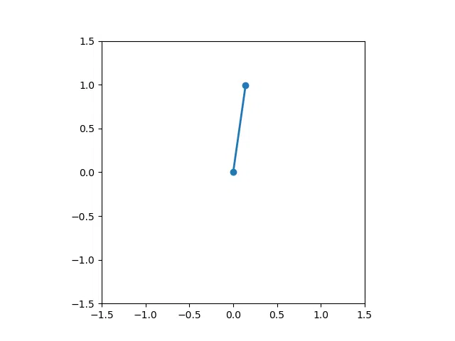
Figure 4. Single pendulum system.
...
Double Pendulum
Reference: https://gauss.vaniercollege.qc.ca/~iti/proj/2022/Ariel_Vlad.pdf
Let $\theta$ angular displacement from vertical where $0^o$ is down
Kinetic Energy ($T$): Velocity of $m$ is $v=l\dot{\theta}$, so $$ T = {1 \over 2} m_1 v_1^2 + {1 \over 2} m_2 v_2^2 = {1 \over 2} m_1 l_1^2 \dot{\theta}_1^2 + {1 \over 2} m_2 ( l_1^2 \dot{\theta}_1^2 + l_2^2 \dot{\theta}_2^2 + 2 l_1 l_2 \dot{\theta}_1 \dot{\theta}_2 cos(\theta_1 - \theta_2)) $$
Potential Energy ($U$): $$ U = -(m_1 + m_2) g l_1 (cos \theta_1) - m_2 g l_2 (cos \theta_2) $$
Lagrangian ($L=T-U$): $$ L = {1 \over 2} m_1 l_1^2 \dot{\theta}_1^2 + {1 \over 2} m_2 ( l_1^2 \dot{\theta}_1^2 + l_2^2 \dot{\theta}_2^2 + 2 l_1 l_2 \dot{\theta}_1 \dot{\theta}_2 cos(\theta_1 - \theta_2)) + (m_1 + m_2) g l_1 (cos \theta_1) - m_2 g l_2 (cos \theta_2) $$
Euler-Lagrange: ${d \over dt} ({\delta L \over \delta \dot{\theta}}) - {{\delta L} \over {\delta \theta}} = 0$ $$ {\delta L \over \delta \dot{\theta}} = TBC, \ {d \over dt} ({\delta L \over \delta \dot{\theta}}) = TBC, \ {{\delta L} \over {\delta \theta}} = TBC \theta $$
So, $$ (m_1 + m_2)l_1 \ddot{\theta}_1 + m_2l_2\ddot{\theta}_2 cos(\theta_1 - \theta_2) + m_2l_2(\dot{\theta}_2)^2 sin(\theta_1 - \theta_2) + g(m_1 + m_2)sin \theta_1 = 0 $$
$$ l_2 \ddot{\theta}_1 cos(\theta_1 - \theta_2) - l_1 (\dot{\theta}_1)^2 sin(\theta_1 - \theta_2) + g sin \theta_2 = 0 $$
$$ $$
General nonlinear form: $$ \begin{bmatrix} (m_1 +m_2)l_1 & m_2l_2 cos(\theta_1 - \theta_2)\\ l_1 cos(\theta_1 - \theta_2) & l_2 \end{bmatrix} \begin{bmatrix} \dot \omega_1 \\ \dot \omega_2 \end{bmatrix} + \begin{bmatrix} m_2l_2(\omega_2)^2 sin(\theta_1 - \theta_2) + g(m_1 + m_2)sin \theta_1 \\ -l_1(\omega_1)^2 sin(\theta_1 - \theta_2) + g sin \theta_2 \end{bmatrix} = 0 $$
Linear approximation assuming small angles: $$ \begin{bmatrix} (m_1 +m_2)l_1 & m_2l_2 \\l_1 & l_2 \end{bmatrix} \begin{bmatrix} \dot \omega_1 \\ \dot \omega_2 \end{bmatrix} + \begin{bmatrix} m_2l_2 + 0 \\ 0 + g \end{bmatrix} \begin{bmatrix} \theta_1 \\ \theta_2 \end{bmatrix}= 0 $$
Show code
def derivatives_double_pendulum(state, const):

    theta1, omega1, theta2, omega2 = state
    g, l1, l2, m1, m2 = const

    a11 = (m1 + m2) *l1
    a12 = m2 * l2* np.cos(theta1 - theta2)
    b1  = m2 * l2 * omega2**2 * np.sin(theta1 - theta2) + g * (m1 + m2) * np.sin(theta1)

    a21 = l1 * np.cos(theta1 - theta2)
    a22 = l2
    b2  = -l1 * omega1**2 * np.sin(theta1 - theta2) + g * np.sin(theta2)

    A = np.array([[a11, a12],[a21, a22]])
    B = np.array([[b1],[b2]])

    x = np.dot(np.linalg.inv(A), -B)

    dtheta1 = omega1
    domega1 = x[0].item()
    dtheta2 = omega2
    domega2 = x[1].item()

    return [dtheta1, domega1, dtheta2, domega2]
Show code
# Run double pendulum solution
initial_state_double = [3, 0, 3, 0]     # theta1, omega1, theta2, omega2
constants_double = [9.81, 2, 1, 1, 1]   # g, l1, l2, m1, m2

times, double_solution = ODE_to_solve(initial_state_double, dt, t_end, ODE_method_rk4,
                                      derivatives_double_pendulum, constants_double)

x1_data_double_solution = constants_double[1]*np.sin(double_solution[:, 0])[::frame_loss]
y1_data_double_solution = -constants_double[1]*np.cos(double_solution[:, 0])[::frame_loss]
x2_data_double_solution = x1_data_double_solution + constants_double[2]*np.sin(double_solution[:, 2])[::frame_loss]
y2_data_double_solution = y1_data_double_solution - constants_double[2]*np.cos(double_solution[:, 2])[::frame_loss]
Show code
# Animate pendulums

fig, ax = plt.subplots()

ax.autoscale = False
ax.set_xlim(-3.5, 3.5)
ax.set_ylim(-3.5, 3.5)
ax.set_aspect('equal')
# ax[0, 0].grid(False)
# ax[0, 0].set_axis_off()

line_double1,  = ax.plot([], [], 'o-', lw=2)
line_double2,  = ax.plot([], [], 'o-', lw=2)

def init():
    line_double1.set_data([], [])
    line_double2.set_data([], [])

    return line_double1, line_double2

def animate(i):

    x1_double = [0, x1_data_double_solution[i]]
    y1_double = [0, y1_data_double_solution[i]]
    x2_double = [x1_data_double_solution[i], x2_data_double_solution[i]]
    y2_double = [y1_data_double_solution[i], y2_data_double_solution[i]]

    line_double1.set_data(x1_double, y1_double)
    line_double2.set_data(x2_double, y2_double)

    return line_double1, line_double2

ani = animation.FuncAnimation(fig, animate, frames=len(x_data_single_solution),
                              interval = frame_loss, blit = True, init_func=init)

plt.close(fig)
ani.save('assets/images/pendulum_double_ani.webp', writer='pillow', fps=20)
# HTML(ani.to_jshtml())
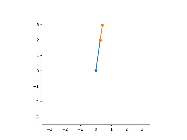
Figure 5. Double pendulum system.
...
Inverted pendulum on cart
Lagrangian ($L=T-U$): For a pendulum from above: $$ L = {1 \over 2} m l^2 \dot{\theta}^2 - m g l (1 - cos \theta) $$
Add the cart of mass $M$ moving in the $x$ axis: $$ L = {1 \over 2} (M + m) \dot{x}^2 - m l \dot{x} cos \theta + {1 \over 2} m l^2 \dot{\theta}^2- m g l (1 - cos \theta) $$
Euler-Lagrange: ${d \over dt} ({\delta L \over \delta \dot{\theta}}) - {{\delta L} \over {\delta \theta}} = 0$, ${d \over dt} ({\delta L \over \delta \dot{x}}) - {{\delta L} \over {\delta x}} = F$
$$ F = (M + m) \ddot x - m l \ddot \theta cos \theta + m l \dot \theta ^2 sin \theta $$ $$ 0 = l \ddot \theta - g sin \theta + \ddot x cos \theta $$
XXX $$ \begin{bmatrix} F \\ 0 \end{bmatrix} = \begin{bmatrix} (M + m) & ml cos\theta \\ cos\theta & l \end{bmatrix} \begin{bmatrix} \ddot x \\ \ddot \theta \end{bmatrix} + \begin{bmatrix} ml \dot\theta^2 sin\theta \\ -gsin\theta \end{bmatrix} $$
Show code
def derivatives_single_trolly(state, const):

    theta, omega, x, v, F = state
    g, l, M, m = const

    a11 = (M + m)
    a12 = m * l * np.cos(theta)
    b1  = m * l * omega**2 * np.sin(theta)

    a21 = np.cos(theta)
    a22 = l
    b2  = -g * np.sin(theta)

    A = np.array([[a11, a12],[a21, a22]])
    B = np.array([[b1],[b2]])
    y = np.array([[F], [0]])

    x = np.dot(np.linalg.inv(A), (y - B))

    dx     = v
    ddx    = x[0].item()
    dtheta = omega
    domega = x[1].item()
    dF     = 0

    return [dtheta, domega, dx, ddx, dF]
Show code
# Run single inverted pendulum on cart
initial_state_inverted = [0.5, 0, 0, 0, 0] # theta, omega, x, v, F
constants_inverted = [9.81, 2, 10, 1] # g, l, M, m

times, inverted_solution = ODE_to_solve(initial_state_inverted, dt, t_end, ODE_method_rk4,
                                        derivatives_single_trolly, constants_inverted)

cart_data_inverted = inverted_solution[:, 3][::frame_loss]
x_data_inverted = constants_inverted[1]*np.sin(inverted_solution[:, 0])[::frame_loss]
y_data_inverted = constants_inverted[1]*np.cos(inverted_solution[:, 0])[::frame_loss]
Show code
# Animate pendulums

fig, ax = plt.subplots()

ax.autoscale = False
ax.set_xlim(-4.5, 4.5)
ax.set_ylim(-3.5, 3.5)
ax.set_aspect('equal')
# ax[0, 0].grid(False)
# ax[0, 0].set_axis_off()

line_invert,   = ax.plot([], [], 'o-', lw=2)

cart_width = 1.2
cart_height = 0.6

def anchor_from_center(xy_center, width, height):
    x_anchor = xy_center[0] - width / 2
    y_anchor = xy_center[1] - height / 2
    return [x_anchor, y_anchor]

cart_single = patches.Rectangle(anchor_from_center([0, 0], cart_width, cart_height),
                                cart_width, cart_height, facecolor = "grey")

ax.add_patch(cart_single)

def init():

    line_invert.set_data([], [])


    cart_single.set_xy(anchor_from_center([0, 0], cart_width, cart_height))

    return cart_single,

def animate(i):

    x_invert = [cart_data_inverted[i], cart_data_inverted[i] + x_data_inverted[i]]
    y_invert = [0, y_data_inverted[i]]

    line_invert.set_data(x_invert, y_invert)

    cart_single.set_xy(anchor_from_center([cart_data_inverted[i], 0], cart_width, cart_height))

    return cart_single,

ani = animation.FuncAnimation(fig, animate, frames=len(x_data_single_solution),
                              interval = frame_loss, blit = True, init_func=init)

plt.close(fig)
ani.save('assets/images/pendulum_invert_ani.webp', writer='pillow', fps=20)
# HTML(ani.to_jshtml())
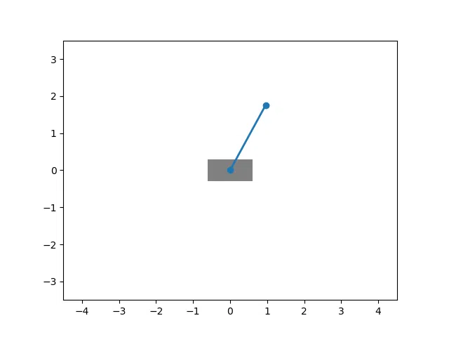
Figure 6. Inverted pendulum on cart.
...
Double inverted pendulum on cart
Reference: https://www3.math.tu-berlin.de/Vorlesungen/SS12/Kontrolltheorie/matlab/inverted_pendulum.pdf
$$ \begin{bmatrix} F \\ 0 \\ 0\end{bmatrix} = \begin{bmatrix} M + m_1 + m_2 & (m_1 + m_2) l_1 cos\theta_1 & m_2l_2cos\theta_2 \\ l_1(m_1 + m_2)cos\theta_1 & l^2_1(m_1 + m_2) & l_1l_2m_2cos(\theta_1 - \theta_2) \\ l_2m_2cos\theta_2 & l_1l_2m_2cos(\theta_1-\theta_2) & l^2_2m_2 \end{bmatrix} \begin{bmatrix} \ddot x \\ \ddot \theta_1 \\ \ddot \theta_2 \end{bmatrix} + \begin{bmatrix} -l_1(m_1+m_2)\dot\theta_1^2sin\theta_1-m_2l_2\dot\theta_2^2sin\theta_2 \\ l_1l_2m_2\dot\theta^2_2 sin(\theta_1 - \theta_2) - g(m_1+m_2)l_1sin\theta_1 \\ -l_1l_2m_2\dot\theta_1^2 sin(\theta_1-\theta_2) - l_2m_2gsin\theta_2 \end{bmatrix} $$
Show code
def derivatives_double_trolly(state, const):

    theta1, omega1, theta2, omega2, x, v, F = state
    g, l1, l2, M, m1, m2 = const

    a11 = M + m1 + m2
    a12 = (m1 + m2) * l1 * np.cos(theta1)
    a13 = m2 * l2 * np.cos(theta2)
    b1  = -l1 * (m1 + m2) * omega1**2 * np.sin(theta1) - m2 * l2 * omega2**2 * np.sin(theta2)

    a21 = l2 * (m1 + m2) * np.cos(theta1)
    a22 = l1**2 * (m1 + m2)
    a23 = l1 * l2 * m2 * np.cos(theta1 - theta2)
    b2  = l1 * l2 * m2 * omega2**2 * np.sin(theta1 - theta2) - g * (m1 + m2) * l1 * np.sin(theta1)

    a31 = l2 * m2 * np.cos(theta2)
    a32 = l1 * l2 * m2 * np.cos(theta1 - theta2)
    a33 = l2**2 * m2
    b3  = -l1 * l2 * m2 * omega1**2 * np.sin(theta1 - theta2) - l2 * m2 * g * np.sin(theta2)

    A = np.array([[a11, a12, a13],[a21, a22, a23], [a31, a32, a33]])
    B = np.array([[b1], [b2], [b3]])
    y = np.array([[F], [0], [0]])

    x = np.dot(np.linalg.inv(A), (y - B))

    dx      = v
    ddx     = x[0].item()
    dtheta1 = omega1
    domega1 = x[1].item()
    dtheta2 = omega2
    domega2 = x[2].item()
    dF     = 0

    return [dtheta1, domega1, dtheta2, domega2, dx, ddx, dF]
Show code
# Run double inverted pendulum on cart
initial_state_double_inverted = [0.5, 0, 0.5, 0, 0, 0, 0] # theta1, omega1, theta2, omega2, x, v, F
constants_double_inverted = [9.81, 2, 1, 10, 1, 1]  # g, l1, l2, M, m1, m2

times, double_inverted_solution = ODE_to_solve(initial_state_double_inverted, dt, t_end, ODE_method_rk4,
                                               derivatives_double_trolly, constants_double_inverted)

cart_data_dinverted = double_inverted_solution[:, 4][::frame_loss]
x1_data_dinverted = constants_double_inverted[1]*np.sin(double_inverted_solution[:, 0])[::frame_loss]
y1_data_dinverted = constants_double_inverted[1]*np.cos(double_inverted_solution[:, 0])[::frame_loss]
x2_data_dinverted = constants_double_inverted[2]*np.sin(double_inverted_solution[:, 2])[::frame_loss]
y2_data_dinverted = constants_double_inverted[2]*np.cos(double_inverted_solution[:, 2])[::frame_loss]
Show code
# Animate pendulums

fig, ax = plt.subplots()

ax.autoscale = False
ax.set_xlim(-4.5, 4.5)
ax.set_ylim(-3.5, 3.5)
ax.set_aspect('equal')
# ax[0, 0].grid(False)
# ax[0, 0].set_axis_off()

line_dinvert1, = ax.plot([], [], 'o-', lw=2)
line_dinvert2, = ax.plot([], [], 'o-', lw=2)

cart_width = 1.2
cart_height = 0.6

def anchor_from_center(xy_center, width, height):
    x_anchor = xy_center[0] - width / 2
    y_anchor = xy_center[1] - height / 2
    return [x_anchor, y_anchor]

cart_double = patches.Rectangle(anchor_from_center([0, 0], cart_width, cart_height),
                                cart_width, cart_height, facecolor = "grey")

ax.add_patch(cart_double)

def init():
    line_dinvert1.set_data([], [])
    line_dinvert2.set_data([], [])

    cart_double.set_xy(anchor_from_center([0, 0], cart_width, cart_height))

    return cart_double,

def animate(i):

    x1_dinvert = [cart_data_dinverted[i], cart_data_dinverted[i] + x1_data_dinverted[i]]
    y1_dinvert = [0, y1_data_dinverted[i]]
    x2_dinvert = [cart_data_dinverted[i] + x1_data_dinverted[i], cart_data_dinverted[i] + x1_data_dinverted[i] + x2_data_dinverted[i]]
    y2_dinvert = [y1_data_dinverted[i], y1_data_dinverted[i] + y2_data_dinverted[i]]

    line_dinvert1.set_data(x1_dinvert, y1_dinvert)
    line_dinvert2.set_data(x2_dinvert, y2_dinvert)

    cart_double.set_xy(anchor_from_center([cart_data_dinverted[i], 0], cart_width, cart_height))

    return cart_double,

ani = animation.FuncAnimation(fig, animate, frames=len(x_data_single_solution),
                              interval = frame_loss, blit = True, init_func=init)

plt.close(fig)
ani.save('assets/images/pendulum_dinvert_ani.webp', writer='pillow', fps=20)
# HTML(ani.to_jshtml())
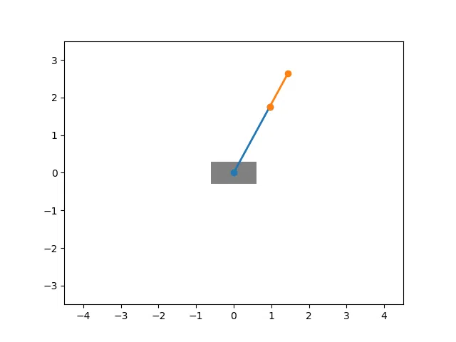
Figure 7. Double inverted pendulum on cart.
...
Simulating the pendulum systems
The following simulates the 4 pendulum systems over 10 seconds.
Show code
# Animate pendulums

fig, ax = plt.subplots(1, 4, figsize=(8, 2))

ax[0].autoscale = False
ax[0].set_xlim(-1.5, 1.5)
ax[0].set_ylim(-1.5, 1.5)
ax[0].set_aspect('equal')
ax[0].grid(False)
ax[0].set_axis_off()

ax[1].autoscale = False
ax[1].set_xlim(-3.5, 3.5)
ax[1].set_ylim(-3.5, 3.5)
ax[1].set_aspect('equal')
ax[1].grid(False)
ax[1].set_axis_off()

ax[2].autoscale = False
ax[2].set_xlim(-4.5, 4.5)
ax[2].set_ylim(-3.5, 3.5)
ax[2].set_aspect('equal')
ax[2].grid(False)
ax[2].set_axis_off()

ax[3].autoscale = False
ax[3].set_xlim(-4.5, 4.5)
ax[3].set_ylim(-3.5, 3.5)
ax[3].set_aspect('equal')
ax[3].grid(False)
ax[3].set_axis_off()

line_single,   = ax[0].plot([], [], 'o-', lw=2)
line_double1,  = ax[1].plot([], [], 'o-', lw=2)
line_double2,  = ax[1].plot([], [], 'o-', lw=2)
line_invert,   = ax[2].plot([], [], 'o-', lw=2)
line_dinvert1, = ax[3].plot([], [], 'o-', lw=2)
line_dinvert2, = ax[3].plot([], [], 'o-', lw=2)

cart_width = 1.2
cart_height = 0.6

def anchor_from_center(xy_center, width, height):
    x_anchor = xy_center[0] - width / 2
    y_anchor = xy_center[1] - height / 2
    return [x_anchor, y_anchor]

cart_single = patches.Rectangle(anchor_from_center([0, 0], cart_width, cart_height),
                                cart_width, cart_height, facecolor = "grey")
cart_double = patches.Rectangle(anchor_from_center([0, 0], cart_width, cart_height),
                                cart_width, cart_height, facecolor = "grey")

ax[2].add_patch(cart_single)
ax[3].add_patch(cart_double)

def init():
    line_single.set_data([], [])
    line_double1.set_data([], [])
    line_double2.set_data([], [])
    line_invert.set_data([], [])
    line_dinvert1.set_data([], [])
    line_dinvert2.set_data([], [])

    cart_single.set_xy(anchor_from_center([0, 0], cart_width, cart_height))
    cart_double.set_xy(anchor_from_center([0, 0], cart_width, cart_height))

    return line_single, line_double1, line_double2, line_invert, line_dinvert1, line_dinvert2, cart_single, cart_double

def animate(i):
    x_single = [0, x_data_single_solution[i]]
    y_single = [0, y_data_single_solution[i]]

    x1_double = [0, x1_data_double_solution[i]]
    y1_double = [0, y1_data_double_solution[i]]
    x2_double = [x1_data_double_solution[i], x2_data_double_solution[i]]
    y2_double = [y1_data_double_solution[i], y2_data_double_solution[i]]

    x_invert = [cart_data_inverted[i], cart_data_inverted[i] + x_data_inverted[i]]
    y_invert = [0, y_data_inverted[i]]

    x1_dinvert = [cart_data_dinverted[i], cart_data_dinverted[i] + x1_data_dinverted[i]]
    y1_dinvert = [0, y1_data_dinverted[i]]
    x2_dinvert = [cart_data_dinverted[i] + x1_data_dinverted[i], cart_data_dinverted[i] + x1_data_dinverted[i] + x2_data_dinverted[i]]
    y2_dinvert = [y1_data_dinverted[i], y1_data_dinverted[i] + y2_data_dinverted[i]]

    line_single.set_data(x_single, y_single)
    line_double1.set_data(x1_double, y1_double)
    line_double2.set_data(x2_double, y2_double)
    line_invert.set_data(x_invert, y_invert)
    line_dinvert1.set_data(x1_dinvert, y1_dinvert)
    line_dinvert2.set_data(x2_dinvert, y2_dinvert)

    cart_single.set_xy(anchor_from_center([cart_data_inverted[i], 0], cart_width, cart_height))
    cart_double.set_xy(anchor_from_center([cart_data_dinverted[i], 0], cart_width, cart_height))

    return line_single, line_double1, line_double2, line_invert, line_dinvert1, line_dinvert2, cart_single, cart_double

plt.tight_layout(pad=0.0)

ani = animation.FuncAnimation(fig, animate, frames=len(x_data_single_solution),
                              interval = frame_loss, blit = True, init_func=init)

plt.close(fig)
ani.save('assets/images/pendulum_ani.webp', writer='pillow', fps=20)
# HTML(ani.to_jshtml())
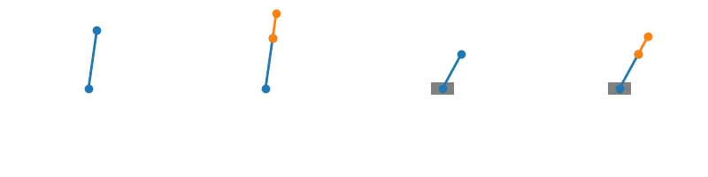
Figure 8. Animation of 4 pendulum systems.
...
Chaos plot
The following demonstrates the chaotic motion of a double pendulum.
Show code
# Run double pendulum solution

dt = 0.001
t_end = 60
frame_loss = 100

initial_state_chaos = [3, 0, 3, 0]     # theta1, omega1, theta2, omega2
constants_chaos = [9.81, 2, 1, 2, 1]   # g, l1, l2, m1, m2

times, chaos_solution = ODE_to_solve(initial_state_double, dt, t_end, ODE_method_rk4,
                                      derivatives_double_pendulum, constants_double)

x1_data_chaos_solution = constants_chaos[1]*np.sin(chaos_solution[:, 0])[::frame_loss]
y1_data_chaos_solution = -constants_chaos[1]*np.cos(chaos_solution[:, 0])[::frame_loss]
x2_data_chaos_solution = x1_data_chaos_solution + constants_chaos[2]*np.sin(chaos_solution[:, 2])[::frame_loss]
y2_data_chaos_solution = y1_data_chaos_solution - constants_chaos[2]*np.cos(chaos_solution[:, 2])[::frame_loss]
Show code
# Plot chaos
fig, ax = plt.subplots(figsize=(6,6))

ax.autoscale = False
ax.set_xlim(-3.5, 3.5)
ax.set_ylim(-3.5, 3.5)
ax.set_aspect('equal')
ax.grid(False)
ax.set_axis_off()

line_double1,  = ax.plot([], [], 'o-', lw=2)
line_double2,  = ax.plot([], [], 'o-', lw=2)
line,  = ax.plot([], [], ':', lw=1)

def init():

    line_double1.set_data([], [])
    line_double2.set_data([], [])
    line.set_data([], [])

    return line_double1, line_double2, line

def animate(i):

    x1_double = [0, x1_data_chaos_solution[i]]
    y1_double = [0, y1_data_chaos_solution[i]]
    x2_double = [x1_data_chaos_solution[i], x2_data_chaos_solution[i]]
    y2_double = [y1_data_chaos_solution[i], y2_data_chaos_solution[i]]

    line_double1.set_data(x1_double, y1_double)
    line_double2.set_data(x2_double, y2_double)

    line.set_data(x2_data_chaos_solution[0:i], y2_data_chaos_solution[0:i])

    return line_double1, line_double2, line

plt.tight_layout(pad=0.0)

ani = animation.FuncAnimation(fig, animate, frames=len(x1_data_chaos_solution),
                              interval = frame_loss, blit = True, init_func=init)

plt.close(fig)
ani.save('assets/images/chaos_ani.webp', writer='pillow', fps=30)
# HTML(ani.to_jshtml())
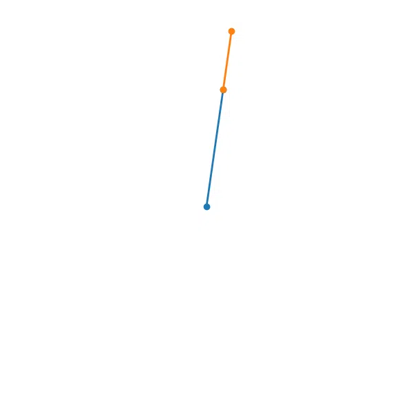
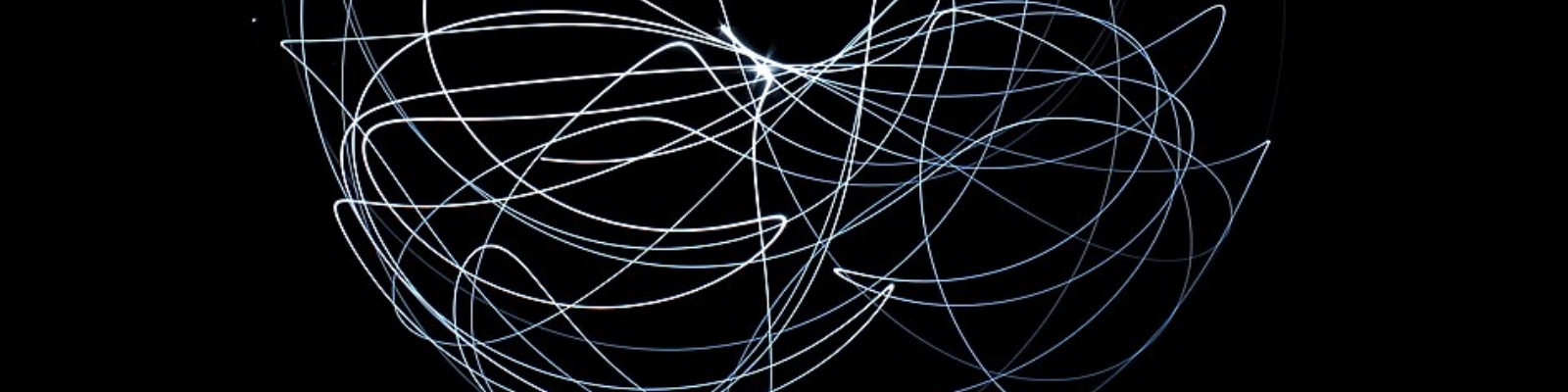
Figure 9. Chaotic path of a double pendulum.
...